Have you ever watched a robot arm in an industrial setting precisely pick up a component with fluid, seamless motion? Behind that elegance lies a mathematical framework called Kinematics. Calculating the end-effector (EE) position from each joint angle is called forward kinematics; working backwards from a desired position to find the joint angles is inverse kinematics. In this article, we explain DH parameters, the Jacobian matrix, and the concept of singularity with concrete examples, and introduce how to use the Robot Arm FK/IK Calculator — a tool you can run directly in your browser.
Why Is Robot Kinematics Hard?
The most disorienting thing when first studying robot kinematics is that the formulas themselves seem simple, yet applying them in practice rarely goes as expected. When I first worked on path planning for a 6-axis vertical articulated robot, the forward kinematics came together quickly — but the inverse kinematics would sometimes spin joints by 1000 degrees, or diverge entirely for positions that were clearly reachable. The culprit turned out to be numerical instability near singularities, and that was the moment I understood that kinematics is far more than matrix multiplication.
There are three main reasons robot kinematics is difficult. First, coordinate transformations stack sequentially. For a 6-DOF robot, you must multiply six 4×4 homogeneous transformation matrices in order to obtain the final EE pose. Second, inverse kinematics can yield multiple solutions or no solution at all. For the same target position, there may simultaneously exist an Elbow Up solution and an Elbow Down solution. Third, near singularities, the problem becomes numerically unstable, causing serious control issues.
Denavit–Hartenberg Parameters: The Starting Point of All Kinematics
The most standard way to mathematically describe the structure of a robot arm is via Denavit–Hartenberg (DH) parameters. Proposed by Denavit and Hartenberg in 1955, this representation defines each link using four parameters.
| Parameter | Symbol | Meaning |
|---|---|---|
| Link length | a | Length of the common normal between adjacent joint Z-axes |
| Link twist | α | Angle between adjacent joint Z-axes |
| Joint angle | θ | Angle between common normals (variable for revolute joints, fixed for prismatic joints) |
| Link offset | d | Distance between common normals (variable for prismatic joints, fixed for revolute joints) |
Applying these four parameters to a single link yields a 4×4 homogeneous transformation matrix:
The full forward kinematics of a robot is obtained by multiplying these matrices in sequence from the base to the EE:
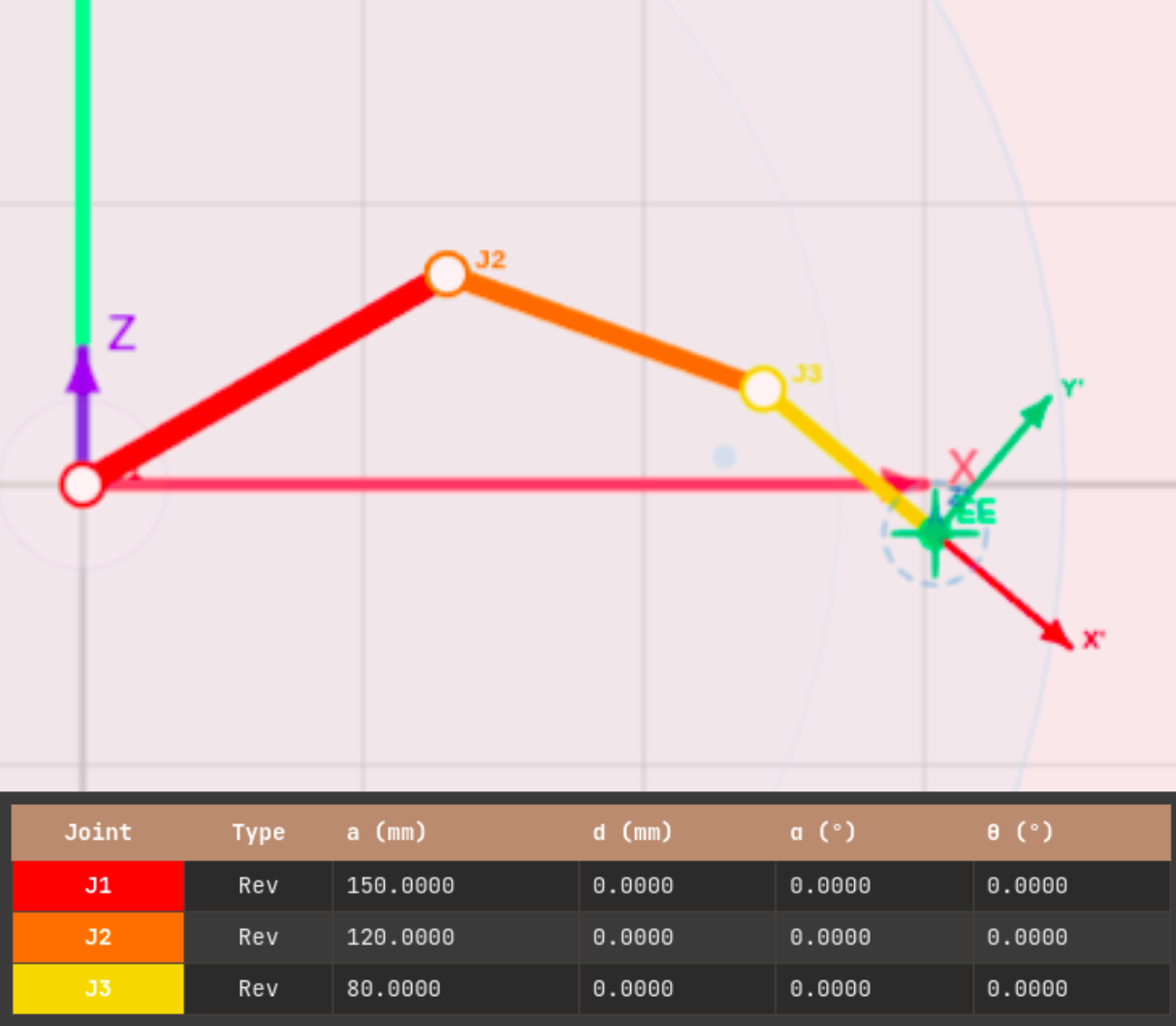
DH parameter table example: 3-DOF planar robot. Each row defines one link; both revolute (Rev) and prismatic (Pri) joints can be represented.
The strength of DH parameters is that any serial robot structure can be expressed in the same format. SCARA, 6-axis vertical articulated, Cartesian robots, and even custom structures of your own design can all be described with a DH table. Universal Robots' publicly available UR series DH parameter documentation is an excellent reference for seeing how DH parameters are applied to real industrial robots.
Forward Kinematics (FK): Computing EE Pose from Joint Angles
Forward kinematics is the problem of finding the position and pose of the EE given the variables of each joint (θ or d). Mathematically, it is completely solved by the matrix multiplication described above, and the solution always exists and is unique. The upper-left 3×3 submatrix of the resulting 4×4 matrix gives the rotation matrix (EE orientation), while the top three elements of the last column give the position vector (X, Y, Z).
One important practical note: maintain consistent units for angles (radians vs. degrees) and lengths (mm vs. m). Mixing them causes unexpected scaling errors in the DH matrix computation.
FK Use Cases
Education and verification: When checking simulation results against hand calculations. For example, compute the EE position for a 2-DOF planar robot at θ₁=30°, θ₂=45° directly via DH matrices and compare against the simulator output.
Path planning: When performing joint-space linear interpolation and tracking the actual EE trajectory. A straight line in joint space traces a curve in Cartesian space.
Inverse Kinematics (IK): Back-Calculating Joint Angles from a Target Position
Inverse kinematics is the problem of finding the joint angles that achieve a desired EE position (and orientation). Unlike forward kinematics, there may be multiple solutions, no solution at all, and the problem is numerically far more demanding. Solution methods fall into two broad categories.
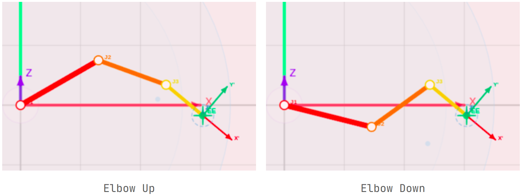
Two inverse kinematics solutions for the same target position: Elbow Up and Elbow Down. In practice, joint limits and collision avoidance must be considered when selecting one.
Analytical vs. Numerical Solutions
Analytical (closed-form) solutions use geometric relationships to directly derive joint angles in explicit mathematical form. They are only possible for 2-DOF/3-DOF planar robots or specific 6-axis robots with simple wrist structures. The advantages are fast computation and the ability to enumerate all solutions explicitly.
Numerical solutions converge to a solution through iteration. The most widely used method is the Damped Least Squares (DLS) Jacobian method. It can be applied to any robot structure and is practical because joint limits and collision avoidance can be added as constraints. Middleware like MoveIt! internally uses iterative IK solvers of this kind.
Here, λ is the damping factor. When the determinant of (JJ^T) approaches zero near a singularity, λ prevents the matrix inverse from diverging. If λ is too large, the step toward the target becomes small and convergence is slow; if too small, joint velocities explode near singularities. In practice, adaptive methods that adjust λ based on current error magnitude or manipulability are commonly used.
The Importance of Initial Value Strategy
With numerical IK, the solution that the algorithm converges to depends on the initial joint angles (the seed). Common strategies include:
- Current joint angles: Favorable for maintaining smooth continuity in real-time control
- Zero seed: Searches from a reference pose, yielding high reproducibility
- Random initial values: Broadens the search space when multiple solutions exist
In practice, a multi-seed strategy — computing solutions from several initial values and selecting the one with the smallest position error — is frequently used.
Jacobian Matrix and Singularity: The Most Critical Concept
The Jacobian matrix is a central tool in robot kinematics. Mathematically, it is a 6×N matrix that linearly relates EE velocity to joint velocity (6 rows: 3 for linear velocity + 3 for angular velocity; N: number of joints):
The Jacobian has two key applications.
Inverse kinematics computation: In the DLS method described above, J transforms the EE position error into a joint angle correction.
Manipulability evaluation: Based on the Manipulability Ellipsoid concept proposed by Yoshikawa in 1985, this quantifies how freely the EE can be moved from the current pose:
As w approaches 0, the robot is close to a singularity. At a singularity, the Jacobian's determinant is zero, its inverse does not exist, EE motion in certain directions becomes impossible, and IK fails to converge.
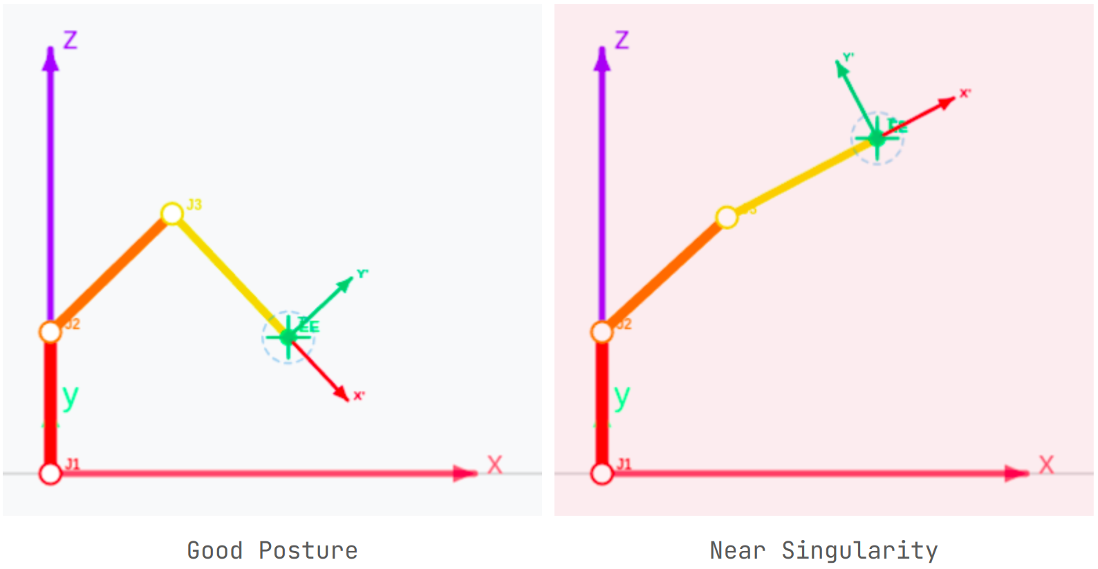
Manipulability ellipsoid: the left (good pose) allows free EE movement in all directions; the right (near singularity) makes movement in certain directions practically impossible.
In industrial settings, singularity issues can lead to serious accidents. If a robot's path is configured to pass near a singularity, joints may instantaneously rotate at extreme velocities, causing mechanical damage or collisions. For this reason, ISO 9283 (Manipulating industrial robots — Performance criteria and related test methods) prescribes robot performance testing procedures and recommends singularity avoidance within the working space, serving as a benchmark for workplace safety design alongside functional safety standards such as IEC 62061 and ISO 13849.
Joint Limits and Practical IK
There is a significant gap between theoretical inverse kinematics and real-world application. The first problem you encounter is joint limits. Real robots have a mechanically defined range of motion for each joint (e.g., J1: ±180°, J2: -90° to +90°).
If joint limits are not incorporated into the IK solver, you end up with poses that are mathematically valid but physically impossible. There are two main approaches to applying joint limits in numerical IK.
Clamping: At each iteration step, if a joint angle exceeds its limit, it is forced back to the boundary value. Simple to implement, but affects convergence speed.
Constrained optimization: Joint limits are formulated as inequality constraints and the problem is solved as a constrained optimization. Theoretically more accurate but significantly more complex to implement.
Angle normalization is also important. Due to accumulated numerical error during iteration, joint angles can grow beyond the -180° to 180° range and reach values like 1000° or more. Applying (θ + 180°) mod 360° − 180° normalization at every step prevents this.
Kinematic Characteristics by Robot Type
2-DOF / 3-DOF Planar Robots
These move only within a plane, so the Z coordinate is always 0. The inverse kinematics can be solved analytically using the law of cosines. The 3-DOF planar robot additionally controls the tool angle (φ). This is the best model to study first for educational purposes.
SCARA Robots
SCARA stands for Selective Compliance Assembly Robot Arm. The structure is compliant in the horizontal direction but rigid in the vertical direction. It was developed by the research team of Professor Hiroshi Makino at the University of Yamanashi in 1978 and commercialized in 1981. It remains widely used today for electronic component assembly and pick-and-place operations. XY-plane positioning is solved analytically in the same way as a 2-DOF planar robot, while the Z height is independently controlled via a prismatic joint (d).
6-DOF Vertical Articulated Robots
The most versatile industrial robot structure. Three main joints determine position; three wrist joints determine orientation. For ideal structures (Spherical Wrist), position and orientation can be decoupled and solved analytically. In the general case, numerical methods are used.
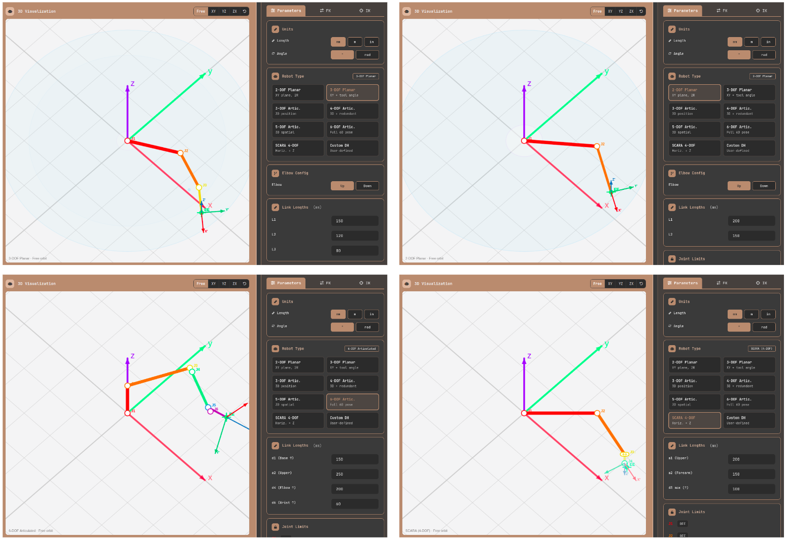
Structural comparison by robot type. Each structure has distinct kinematic properties, leading to different application domains and IK solution methods.
Using an Online IK Calculator: Calculate Directly in the Browser
Once you understand the theory, the fastest way to solidify that understanding is to compute actual numbers yourself. The Robot Arm FK/IK Calculator is an online inverse kinematics calculator and 3D robot arm simulator that runs directly in the browser with no installation required. You can enter DH parameters directly, verify forward kinematics using joint sliders, and input or drag a target position to solve inverse kinematics in real time.
Step 1: Robot Type and Unit Setup
In the Parameters tab, select a robot type (2-DOF planar, 3-DOF planar, SCARA, 4–6 axis articulated, or custom DH) and set link lengths and global units (mm/m/in, degrees/radians). In custom DH mode, you can specify the DOF (2–6) directly and enter a, d, α, θ offset, and joint type (revolute/prismatic) for each link.
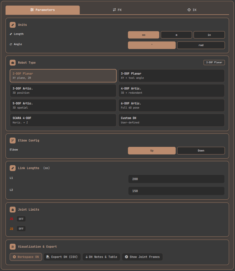
Parameters tab: configure robot type, link lengths, units, and joint limits.
Step 2: Forward Kinematics
Switching to the FK tab reveals per-joint sliders and numeric input fields. Moving a slider updates the 3D canvas in real time, and the result card displays the EE's X, Y, Z position and Roll, Pitch, Yaw orientation. Individual values can be copied to the clipboard using the copy button next to each entry.
Enabling the "Path Trace" feature displays a ghost trail of the EE trajectory on the canvas as you move the sliders. This is particularly useful for directly observing what kind of curve a straight line in joint space traces in Cartesian space.
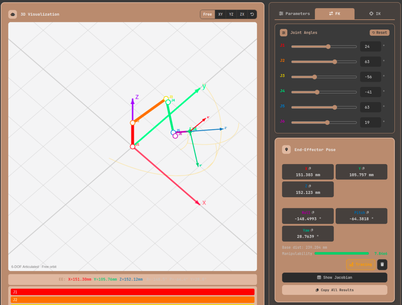
FK tab: moving each joint slider updates the 3D canvas and EE position/orientation results in real time. The Path Trace feature lets you visualize the EE trajectory.
Step 3: Inverse Kinematics and IK Drag
In the IK tab, entering target X, Y, Z values triggers automatic IK computation. Alternatively, you can drag the T marker (target position indicator) on the 3D canvas directly with the mouse. Hovering over the marker reveals a semi-transparent filled circle indicating it is draggable.
Toggling the Jacobian panel button displays the numerical values of the 6×N Jacobian matrix for the current pose. The manipulability indicator bar turns red near singularities, providing an intuitive visual warning about the current pose's risk level.
Latest Trends in Robot Kinematics: Deep Learning IK, Collaborative Robots, and ROS 2
Once you understand the kinematics of each robot type, it is worth knowing how industry is evolving on top of these foundations. Kinematics is a decades-old field, but the way it is applied is changing rapidly.
First, deep learning-based inverse kinematics is being actively researched. Training a neural network to learn complex IK mappings can yield solutions quickly without iterative computation. However, generalization outside the training data distribution and the challenge of enforcing joint limits remain open problems.
Second, the proliferation of collaborative robots (cobots). Cobots such as Universal Robots, FANUC CRX, and ABB GoFa operate in shared spaces with humans, which means kinematic computation must be integrated with real-time safety assessment. Collision detection, force control, and safety zone configuration all operate on top of kinematic calculations.
Third, the maturation of the ROS 2 and MoveIt 2 ecosystem is standardizing kinematic libraries. MoveIt! supports a variety of IK plugins including IKFast, KDL, and TRAC-IK, and can use robot models described in URDF (ROS URDF documentation) directly.
Practical IK Problems for 6-Axis Robots: Singularity, Workspace Limits, and Joint Discontinuity
Here are three problems that frequently arise when implementing pick-and-place tasks with a 6-axis robot.
Problem 1: Wrist Singularity Occurs when J5 (the middle wrist joint) approaches 0°, causing the J4 and J6 axes to align. In this configuration, rotations of J4 and J6 produce identical EE orientation changes, making it impossible to determine their absolute angles independently — the Jacobian loses rank. The solution is to avoid paths that pass through the 0° neighborhood of J5; if unavoidable, apply a small offset to J5 to move away from the singularity.
Problem 2: Workspace Boundary When a target position is very close to the robot's maximum reach or corresponds to an elbow singularity, IK diverges. Workspace boundaries should be visualized during task planning and targets constrained to remain within the reachable region.
Problem 3: Joint Angle Discontinuity When computing IK sequentially for the same target, the solution may abruptly switch from Elbow Up to Elbow Down, causing a large jump in joint angles. Using the previous step's solution as the initial seed (current joint angle seed strategy) makes it easier to maintain continuity.
Closing: Kinematics Is the Language of Robotics
Understanding kinematics thoroughly is like learning the language in which you speak to robots. Forward kinematics reads the robot's current state; inverse kinematics instructs it to perform a desired motion; the Jacobian evaluates how safe and precise that motion is. DH parameters are the common grammar underlying all of this.
I strongly recommend using the Robot Arm FK/IK Calculator alongside your theoretical study to compute real numbers. Enter your own robot structure in custom DH mode, set joint limits, and directly observe how IK converges. In the moment when the manipulability indicator bar turns red near a singularity, the equations in the textbook connect to physical intuition in a way that no lecture can replicate.
References
- Wikipedia, Denavit–Hartenberg parameters — Mathematical definition of DH parameters and derivation of the transformation matrix
- Universal Robots, DH Parameters for Calculations of Kinematics and Dynamics — Publicly available DH parameters for actual industrial robots (UR3/UR5/UR10)
- Wikipedia, Inverse kinematics — Mathematical background and overview of various IK solution methods
- Wikipedia, Jacobian matrix and determinant — Mathematical definition of the Jacobian matrix
- Wikipedia, Manipulability ellipsoid — The manipulability ellipsoid concept and Yoshikawa's manipulability measure
- ISO, ISO 9283:1998 — International standard for manipulating industrial robot performance criteria and test methods
- MoveIt!, moveit.ai — ROS-based robot motion planning framework with support for various IK plugins
- ROS Wiki, URDF — Official documentation for the Unified Robot Description Format